Bioinformatics

Feb

2020

How to read IDF diabetes statistics in Python using Pandas

The International Diabetes Foundation provides a Data portal with various statistics related to diabetes.

In this post we’ll show how to read the Diabetes estimates (20-79 y) / People with diabetes, in 1,000s data export in CSV format using pandas.

First download IDF (people-with-diabetes--in-1-000s).csv from the data page.

Now we can parse the CSV file:

import pandas as pd

# Download at https://www.diabetesatlas.org/data/en/indicators/1/
df = pd.read_csv("IDF (people-with-diabetes--in-1-000s).csv")
# Parse year columns to obtain floats and multiply by thousands factor. Pandas fails to parse values like "12,345.67"
for column in df.columns:
    try:
        int(column)
        df[column] = df[column].apply(lambda s: None if s == "-" else float(s.replace(",", "")) * 1000)
    except:
        pass

As you can see in the postprocessing step, the number of diabetes patients are given in 1000s in the CSV, so we multiply them by 1000 to obtain the actual numbers.

If you want to modify the data columns (i.e. the columns referring to year), you can use this simple template:

for column in df.columns:
    try:
        int(column) # Will raise ValueError() if column is not a year number
        # Whatever you do here will only be applied to year columns
        df[column] = df[column] * 0.75 # Example on how to modify a column
        # But note that if your code raises an Exception, it will be ignored!
    except:
        pass

Let’s plot some data:

regions = df[df["Type"] == "Region"] # Only regions, not individual countries

from matplotlib import pyplot as plt
plt.style.use("ggplot")
plt.gcf().set_size_inches(20,4)
plt.ylabel("Diabetes patients [millions]")
plt.xlabel("Region")
plt.title("Diabetes patients in 2019 by region")
plt.bar(regions["Country/Territory"], regions["2019"] / 1e6)

Note that if you use a more recent dataset than the version I’m using the 2019 column might not exist in your CSV file. Choose an appropriate column in that case.

Feb

2020

Parsing World Population Prospects (WPP) XLSX data in Python

The United Nations provides the Word Population Prospects (WPP) dataset on geographic and age distribution of mankind as downloadable XLSX files.

Reading these files in Python is rather easy. First we have to find out how many rows to skip. For the 2019 WPP dataset this value is 16 since row 17 contains all the column headers. The number of rows to skip might be different depending on the dataset. We’re using WPP2019_POP_F07_1_POPULATION_BY_AGE_BOTH_SEXES.xlsx in this example.

We can use Pandas read_excel() function to import the dataset in Python:

import pandas as pd

df = pd.read_excel("WPP2019_INT_F03_1_POPULATION_BY_AGE_ANNUAL_BOTH_SEXES.xlsx", skiprows=16, na_values=["..."])

This will take a few seconds until the large dataset has been processed. Now we can check if skiprows=16 is the correct value. It is correct if pandas did recognize the column names correctly:

>>> df.columns
Index(['Index', 'Variant', 'Region, subregion, country or area *', 'Notes',
       'Country code', 'Type', 'Parent code', 'Reference date (as of 1 July)',
       '0-4', '5-9', '10-14', '15-19', '20-24', '25-29', '30-34', '35-39',
       '40-44', '45-49', '50-54', '55-59', '60-64', '65-69', '70-74', '75-79',
       '80-84', '85-89', '90-94', '95-99', '100+'],
      dtype='object')

Now let’s filter for a country:

russia = df[df["Region, subregion, country or area *"] == 'Russian Federation']

This will show us the population data for multiple years in 5-year intervals from 1950 to 2020. Now let’s filter for the most recent year:

russia.loc[russia["Reference date (as of 1 July)"].idxmax()]

This will show us a single dataset:

Index                                                 3255
Variant                                          Estimates
Region, subregion, country or area *    Russian Federation
Notes                                                  NaN
Country code                                           643
Type                                          Country/Area
Parent code                                            923
Reference date (as of 1 July)                         2020
0-4                                                9271.69
5-9                                                9350.92
10-14                                              8174.26
15-19                                              7081.77
20-24                                               6614.7
25-29                                              8993.09
30-34                                              12543.8
35-39                                              11924.7
40-44                                              10604.6
45-49                                              9770.68
50-54                                              8479.65
55-59                                                10418
60-64                                              10073.6
65-69                                              8427.75
70-74                                              5390.38
75-79                                              3159.34
80-84                                              3485.78
85-89                                              1389.64
90-94                                              668.338
95-99                                              102.243
100+                                                 9.407
Name: 3254, dtype: object

How can we plot that data? First, we need to select all the columns that contain age data. We’ll do this by manually inserting the name of the first such column (0-4) into the following code and assuming that there are no columns after the last age column:

>>> df.columns[df.columns.get_loc("0-4"):]
Index(['0-4', '5-9', '10-14', '15-19', '20-24', '25-29', '30-34', '35-39',
       '40-44', '45-49', '50-54', '55-59', '60-64', '65-69', '70-74', '75-79',
       '80-84', '85-89', '90-94', '95-99', '100+'],
      dtype='object')

Now let’s select those columns from the russia dataset:

most_recent_russia = russia.loc[russia["Reference date (as of 1 July)"].idxmax()]
age_columns = df.columns[df.columns.get_loc("0-4"):]

russian_age_data = most_recent_russia[age_columns]

Let’s have a look at the dataset:

>>> russian_age_data
0-4      9271.69
5-9      9350.92
10-14    8174.26
15-19    7081.77
20-24     6614.7
25-29    8993.09
30-34    12543.8
35-39    11924.7
40-44    10604.6
45-49    9770.68
50-54    8479.65
55-59      10418
60-64    10073.6
65-69    8427.75
70-74    5390.38
75-79    3159.34
80-84    3485.78
85-89    1389.64
90-94    668.338
95-99    102.243
100+       9.407

That looks useable, note however that the values are in thousands, i.e. we have to multiply the values by 1000 to obtain the actual estimates of the population. Let’s plot it:

from matplotlib import pyplot as plt
plt.style.use("ggplot")

plt.title("Age composition of the Russian population (2020)")
plt.ylabel("People in age group [Millions]")
plt.xlabel("Age group")
plt.gcf().set_size_inches(15,5)
# Data is given in thousands => divide by 1000 to obtain millions
plt.plot(russian_age_data.index, russian_age_data.as_matrix() / 1000., lw=3)

The finished plot will look like this:

Here’s our finished script:

#!/usr/bin/env python3
import pandas as pd
df = pd.read_excel("WPP2019_POP_F07_1_POPULATION_BY_AGE_BOTH_SEXES.xlsx", skiprows=16)
# Filter only russia
russia = df[df["Region, subregion, country or area *"] == 'Russian Federation']

# Filter only most recent estimate (1 row)
most_recent_russia = russia.loc[russia["Reference date (as of 1 July)"].idxmax()]
# Retain only value columns
age_columns = df.columns[df.columns.get_loc("0-4"):]
russian_age_data = most_recent_russia[age_columns]

# Plot!
from matplotlib import pyplot as plt
plt.style.use("ggplot")

plt.title("Age composition of the Russian population (2020)")
plt.ylabel("People in age group [Millions]")
plt.xlabel("Age group")
plt.gcf().set_size_inches(15,5)
# Data is given in thousands => divide by 1000 to obtain millions
plt.plot(russian_age_data.index, russian_age_data.as_matrix() / 1000., lw=3)

# Export as SVG
plt.savefig("russian-demographics.svg")

Jan

2020

How to map MeSH ID to MeSH term using Python

Our MeSH-JSON project provides a pre-compiled MeSH-ID-to-term map as JSON:

Download here or use this command to download:

wget "http://techoverflow.net/downloads/mesh.json.gz"

How to use in Python:

#!/usr/bin/env python3
import json
import gzip

# How to load
with gzip.open("mesh.json.gz", "rb") as infile:
    mesh_id_to_term = json.load(infile)

# Usage example
print(mesh_id_to_term["D059630"]) # Prints 'Mesenchymal Stem Cells'

Jan

2020

How to download & sync PubMed baseline + updates

In our previous post How to download PubMed baseline data using rsync we showed how you can update PubMed’s baseline data. This dataset is only updated yearly – however, you can download the updatefiles which are typically updated once per day.

The commands to download & sync both sets of files into the PubMed directory:

rsync -Pav --delete ftp.ncbi.nlm.nih.gov::pubmed/baseline/\*.xml.gz PubMed/
rsync -Pav --delete ftp.ncbi.nlm.nih.gov::pubmed/updatefiles/\*.xml.gz PubMed/

The --delete option will ensure that files that are deleted on the server will also be deleted locally. For example, when a new baseline dataset is being published, you need to delete the old year’s files to avoid having to process duplicate data.

Jan

2020

How to parse all PubMed baseline files in parallel using Python

In our previous post How to parse PubMed baseline data using Python we investigate how to use the pubmed_parser library to parse PubMed medline data using Python.

In this follow-up we’ll provide an example of how to use glob to select all PubMed baseline files in a directory and use concurrent.futures with tqdm to provide a convenient yet easy-to-use process parallelism using ProcessPoolExecutor and a progress bar UI for the command line.

First, install the requirements using

pip install git+git://github.com/titipata/pubmed_parser.git six numpy tqdm

Now download this script, ensure some files like pubmed20n0002.xml.gz or pubmed20n0004.xml.gz are in the same directory and run it:

#!/usr/bin/env python3
import pubmed_parser as pp
import glob
import os
from collections import Counter
import concurrent.futures
from tqdm import tqdm

# Source: https://techoverflow.net/2017/05/18/how-to-use-concurrent-futures-map-with-a-tqdm-progress-bar/
def tqdm_parallel_map(executor, fn, *iterables, **kwargs):
    """
    Equivalent to executor.map(fn, *iterables),
    but displays a tqdm-based progress bar.
    
    Does not support timeout or chunksize as executor.submit is used internally
    
    **kwargs is passed to tqdm.
    """
    futures_list = []
    for iterable in iterables:
        futures_list += [executor.submit(fn, i) for i in iterable]
    for f in tqdm(concurrent.futures.as_completed(futures_list), total=len(futures_list), **kwargs):
        yield f.result()

def parse_and_process_file(filename):
    """
    This function contains our parsing code. Usually, you would only modify this function.
    """
    # Don't parse authors and references for this example, since we don't need it
    dat = pp.parse_medline_xml(filename, author_list=False, reference_list=False)

    # For this example, we'll build a set of count of all MeSH IDs in this file
    ctr = Counter()
    for entry in dat:
        terms = [term.partition(":")[0].strip() for term in entry["mesh_terms"].split(";")]
        for term in terms:
            ctr[term] += 1
    return filename, ctr


if __name__ == "__main__":
    # Find all pubmed files in the current directory
    all_filenames = glob.glob("pubmed*.xml.gz")
    # For some workloads you might want to use a ThreadPoolExecutor,
    # but a ProcessPoolExecutor is a good default
    executor = concurrent.futures.ProcessPoolExecutor(os.cpu_count())
    # Iterate results as they come in (the order is not the same as in the input!)
    for filename, ctr in tqdm_parallel_map(executor, parse_and_process_file, all_filenames):
        # NOTE: If you print() here, this might interfere with the progress bar,
        # but we accept that here since it's just an example
        print(filename, ctr)

Now you can start modifying the example, most notably the parse_and_process_file() function to do whatever processing you intend to do.

Jan

2020

How to parse PubMed baseline data using Python

Want to parse more than one PubMed file? Also see our follow-up at How to parse all PubMed baseline files in parallel using Python

PubMed provides a data dump of metadata from all PubMed articles on the NCBI Servers.

In this example, we’ll parse one of the compressed metadata XML files using the pubmed_parser Python library.

First, download one of the .xml.gz files. For this example, we’ll use pubmed20n0001.xml.gz.

Now we can install the required libraries:

pip install git+git://github.com/titipata/pubmed_parser.git six numpy

Now you can download & run our script. For this example, we will extract a list of MeSH terms for every and print PubMed ID and a list of MeSH IDs.

#!/usr/bin/env python3
import pubmed_parser as pp

# Don't parse authors and references for this example, since we don't need it
dat = pp.parse_medline_xml("pubmed20n0001.xml.gz", author_list=False, reference_list=False)
# Iterate PubMed entries from that file
for entry in dat:
    # entry["mesh_terms"] is like "D000818:Animal; ..."
    # In this example, we are only interested in the MeSH ID, like D000818.
    # Print the PubMed ID, followed by a list of MeSH terms.
    print(entry["pmid"], [
        term.partition(":")[0].strip() for term in entry["mesh_terms"].split(";")
    ])

Running this script takes 13.3 seconds on my Notebook which is equivalent to about 1.4 MBytes of GZipped input data per second. When running the script, you will see lines like

30957 ['D000319', 'D001794', 'D003864', 'D006801', 'D006973', 'D007676', 'D010869']

which means that the PubMed Article with ID 30957 has the MeSH terms ['D000319', 'D001794', 'D003864', 'D006801', 'D006973', 'D007676', 'D010869'].

See the pubmed_parser documentation, or just try it out interactively for more information on what fields are available in the entries you can iterate.

Jan

2020

How to download PubMed baseline data using rsync

PubMed raw data is hosted on the NCBI servers which provide convenient access using rsync.

Download PubMed baseline data using a rsync command like

rsync -Pav ftp.ncbi.nlm.nih.gov::pubmed/baseline/\*.xml.gz Pubmed/

This example command will download all baseline data files as .xml.gz to the PubMed folder

You can explore the PMC directory structure by accessing the NCBI FTP server using your browser.

Jan

2020

How to download PMC (PubMed Central) bulk data using rsync

PubMed Central (PMC) raw data is hosted on the NCBI servers which provide convenient access using rsync.

Download PMC data using a rsync command like

rsync -Pav ftp.ncbi.nlm.nih.gov::pub/pmc/oa_bulk/\*.tar.gz PMC/

This example command will download all bulk data files as .tar.gz containing text files.

You can explore the PMC directory structure by accessing the NCBI FTP server using your browser.

Jan

2020

Downloading PubChem raw data using rsync

PubChem raw data is hosted on the NCBI servers which provide convenient access using rsync.

Download PubChem data using a rsync command like

rsync -Pav ftp.ncbi.nlm.nih.gov::pubchem/Compound/CURRENT-Full/SDF/\*.gz pubchem/

This example command will download all current compounds in SDF format.

You can explore the PubChem directory structure by accessing the NCBI FTP server using your browser.

Dec

2019

What is Cytarabine Syndrome?

Note about medical information:
This information is presented for informational purposes only and is intended for professionals. While we strive to provide accurate information, this information might be outdated, unintentionally misleading or incorrect. Consult a medical professional and/or read the primary sources cited in our article before basing any decision on this information.

Cytarabine is a cytotoxic agent commonly used in cancer chemotherapy.

A common side-effect of high-dose Cytarabine is called Cytarabine Syndrome which is associated with

Fever
Malaise (discomfort)
Myalgia (muscle pain)
Arthralgia (joint pain)
Conjunctivitis (inflammation of the cornea)
Rashes

Since high-dose cytarabine is associated with myelotoxiticity leading to aplasia and hence immune deficiency due to severe neutropenia, one needs to rule out infectious causes for the fever since these could quickly develop into a clinical emergency (febrile neutropenia). Typically, preemptive treatment with broad-spectrum antibiotics is strongly indicated.

The cause for the cytarabine syndrome is not completely understood but is hypothesized to be general inflammation due to a cytokine release syndrom-like release of pro-inflammatory cytokines due to Cytarabine mediating the apopotosis of large amounts of primarily neoplastic cells.

How common is cytarabine syndrome?

In our reference study, cytarabine syndrome occured in 43% of all HiDAC (high-dose cytarabine) consolidation cycles and 64% of patients had at least one consolidation cycle with cytarabine syndrome.

How long is the duration of the symptoms?

The duration of the fever is rather short (1-72 hours), with a median duration of only 10.5 hours in our reference study.

References:

Gonen et al 2005: Cytarabine-induced fever complicating the clinical course of leukemia

Jirasek et al 2015: Cytarabine syndrome despite corticosteroid premedication in an adult undergoing induction treatment for acute myelogenous leukemia

Castleberry et al 1982: The Cytosine Arabinoside (Ara-C) Syndrome

Bubalo 2015: Prevention and Treatment of Cytarabine-Induced Keratoconjunctivitis

Nov

2019

What is Composite Complete Remission (CRc) in cancer research?

Composite Complete Remission (CRc) is the sum of

Complete Remission (CR), i.e. the primary disease is no longer active and the blood counts have normalized.
Complete Remission with incomplete hematological recovery (CRi), i.e. the primary disease is no longer active but at least one of the blood cell lines has not recovered to normal levels.
Complete Remission with incomplete platelet recovery (CRp), i.e. the primary disease is no longer active but the platelet count has not recovered to normal levels.

Note that some authors include CRp in CRi while others list it separately.

Source: NCT00989261: Efficacy Study for AC220 to Treat Acute Myeloid Leukemia (AML) (ACE) (CRc = CR + CRi) or Cortes et al (2018) (CRc = CR + CRi + CRp)

Example:

If you have a CR rate of $50\%$ and and a CRi rate of $5\%$ , the CRc rate is $50\% + 5\% = 55\%$ .
If you have a CR rate of $50\%$ and and a CRi rate of $4\%$ and a CRp rate or $2\%$ , the CRc rate is $50\% + 4\% + 2\% = 56\%$ .

How is full recovery of the blood cell lines defined?

This depends on the type of primary disease (and sometimes there are slightly conflicting definitions).

For example, Döhner et al (2017) present these numbers for CRi in acute myeloid leukemia:

Neutrophils $\leq \frac{1000}{\mu l}$ (in other words, grade 2 or higher grade neutropenia)
Platelets $\leq \frac{100\,000}{\mu l}$

If these criteria for CRi are not fulfilled (even if the blood counts have not reached normal levels), the state is defined as CR.

Note that in this case there are no limits for erythrocyte count recovery, hence the patient might require blood transfusions due to low levels of hemoglobin even though according to this definition he is considered to be in a state of complete remission (CR).

The meaning of CR as opposed to CRi, CRp or CRc is therefore more relevant as endpoint of a medical study, but not so much as indicator that the patient has recovered to a point that allows discontinuation of treatment.

Also see What is grade I/II/III/IV neutropenia?

Nov

2019

What is grade I/II/III/IV neutropenia?

Neutropenia is a reduced number of neutrophil granulocytes in the blood. Normally, one would expect a number $\geq 1500\ \frac{\text{neutrophils}}{\mu l}$ in the peripheral blood, with a typical value of $2500-4500 \frac{\text{neutrophils}}{\mu l}$ .
The decreased number of neutrophils is associated with reduced immune response and hence causes an increased chance of infection. Patients with neutropenia have a risk of developing febrile neutropenia (also known as neutropenic sepsis). Febrile neutropenia is a medical emergency and hence requires immediate treatment!

Neutropenia can be easily diagnosed using a complete blood count to count the number of neutrophils in the peripheral blood. In case a lab report does not contain the absolute neutrophil count (ANC), you can also multiply the percentage of neutrophils with the leukocyte count.

The different grades of neutropenia are defined in the Common Terminology Criteria for Adverse Events (CTCAE). On this page, we use Version 5.0 published in 2017.

Grade 1 neutropenia

is defined as an absolute neutrophil count (ANC) of

$\leq 1500\ \frac{\text{neutrophils}}{\mu l}$ or equivalently
$\leq 1500\ \frac{\text{neutrophils}}{mm³}$ or equivalently
$\leq 1.5\ billion\ \frac{\text{neutrophils}}{l}$ or equivalently
$\leq 1.5e9\ \frac{\text{neutrophils}}{l}$

Grade 2 neutropenia

is defined as an absolute neutrophil count (ANC) of

$1000\dotsb 1500\ \frac{\text{neutrophils}}{\mu l}$ or equivalently
$1000\dotsb 1500\ \frac{\text{neutrophils}}{mm³}$ or equivalently
$1000\ billion\ \dotsb 1500\ billion\ \frac{\text{neutrophils}}{l}$ or equivalently
$1e9\dotsb 1.5e9\ \frac{\text{neutrophils}}{l}$

Grade 3 neutropenia

is defined as an absolute neutrophil count (ANC) of

$500\dotsb 1000\ \frac{\text{neutrophils}}{\mu l}$ or equivalently
$500\dotsb 1000\ \frac{\text{neutrophils}}{mm³}$ or equivalently
$500\ billion\ \dotsb 1000\ billion\ \frac{\text{neutrophils}}{l}$ or equivalently
$0.5e9\dotsb 1e9\ \frac{\text{neutrophils}}{l}$

Grade 4 neutropenia

is defined as an absolute neutrophil count (ANC) of

$\leq 500\ \frac{\text{neutrophils}}{\mu l}$ or equivalently
$\leq 500\ \frac{\text{neutrophils}}{mm³}$ or equivalently
$\leq 500\ million\ \frac{\text{neutrophils}}{l}$ or equivalently
$\leq 0.5e9\ \frac{\text{neutrophils}}{l}$

Grade 5 neutropenia

is defined as death (like all Grade 5 adverse events).

Nov

2019

What does ‘+ve’ or ‘-ve’ mean in a medical context?

+ve means positive
-ve means negative

Some publishers use these terms instead of just + and - to make clear that the + indicates that a certain parameter is positive or negative, to avoid confusing - with a dash and + with and.

For example, writing p53-ve clearly indicates that p53 is negative. What positive or negative actually means depends on the context, e.g. it can mean that p53 is not mutated in a group of patients. See this paper for an example where p53-ve is used in that way.

Mar

2018

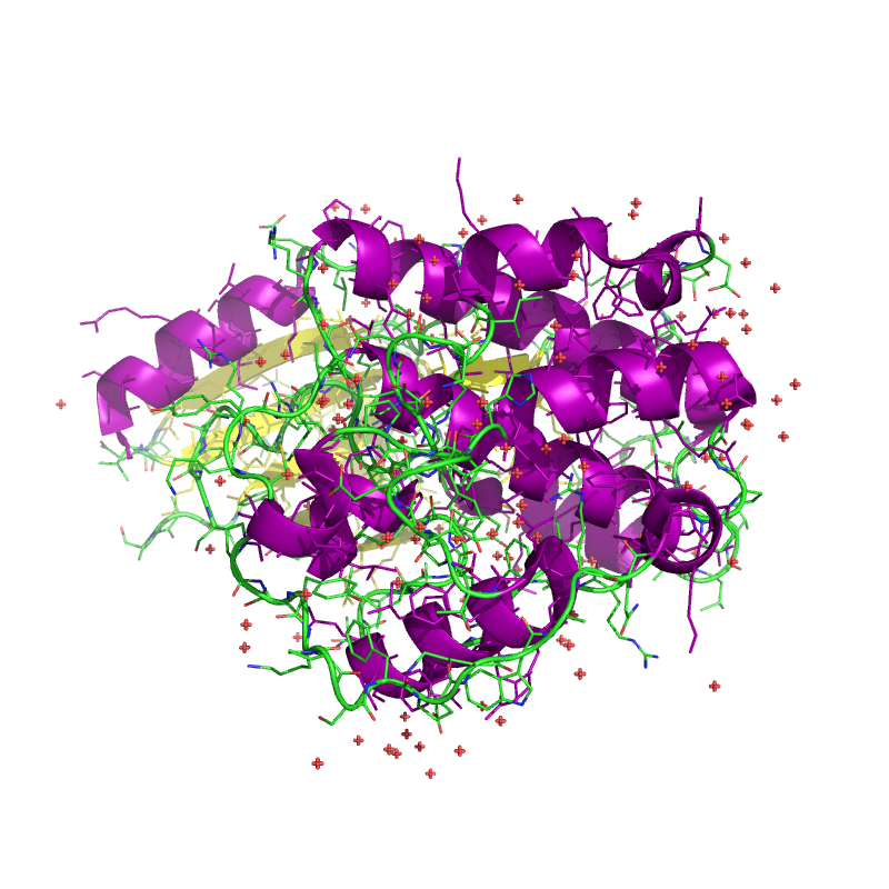
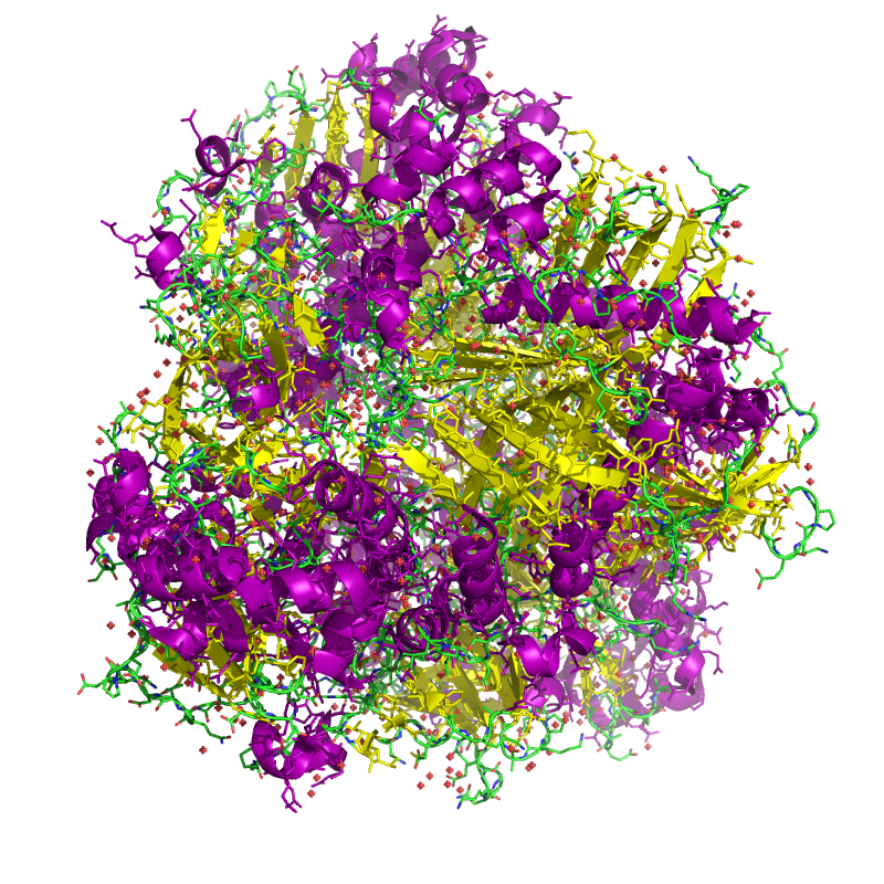
Automated rendering of PDB proteins using PyMol

Downloading the .pdb file

As the RCSB offers direct HTTP acess, this step is trivial.

You can use this shell script to download any protein:

#!/bin/bash
# donwload-pdb.sh
wget http://www.rcsb.org/pdb/files/$1.pdb

Call it with the PDB ID to download, e.g. 1ULI:

./download-pdb.sh 1ULI

Rendering using PyMol

First, install PyMol: Either download it from the website or just use your preferred package manager, e.g.:

sudo apt-get install pymol

By calling PyMol with a script instead of in interactive mode, we can automate the process of rendering an image – manual tuning of the perspective etc is likely to improve the results, however.

The following script integrates both the automatic download and the renderer. A temporary .pml (PyMol script) file is created with static settings

#!/bin/bash
# render-pymol.sh
if [ $# -eq 0 ]
  then
    echo "Usage: render-pymol.sh <PDB ID>"
    exit
fi
#Download
wget -qO $1.pdb http://www.rcsb.org/pdb/files/$1.pdb

#Create the rasmol script
echo "load $1.pdb;" > $1.pml
echo "set ray_opaque_background, on;" >> $1.pml
echo "show cartoon;" >> $1.pml
echo "color purple, ss h;" >> $1.pml
echo "color yellow, ss s;" >> $1.pml
echo "ray 1500,1500;" >> $1.pml
echo "png $1.png;" >> $1.pml
echo "quit;" >> $1.pml

#Execute PyMol
pymol -qxci $1.pml
#Remove temporary files
rm -rf $1.pml $1.pdb

Call it like this:

./render-pymol.sh 1ULI

This command will render the result and store it in 1ULI.png

Customizing the render style

In order to change the size of the generated PNG image, change this line:

echo "ray 1500,1500;" >> $1.pml

The numbers represent the width and height of the generated image. Note that increasing the image size will significantly increase the CPU time required to render the image, especially for complex proteins. Running render-pymol.sh with 1500x1500px to render the 1ULI took 209 seconds on my Notebook as opposed to 33 seconds for 500×500.

These lines define the style of the rendered protein:

echo "show cartoon;" >> $1.pml
echo "color purple, ss h;" >> $1.pml
echo "color yellow, ss s;" >> $1.pml

while this line set the background color to transparent:

echo "set ray_opaque_background, off;" >> $1.pml

If you prefer a white (non-transparent) background instead, you can add this line right after the line containing load $1.pdb:

echo "bg_color white;" >> $1.pml
echo "set ray_opaque_background, off;" >> $1.pml

Results

Feb

2015

Parsing the MeSH ASCII format in Python

Similar to our previously published UniPruot parser, MeSH provides an ASCII format that can easily be parsed using Python.

Just like the UniProt parser, this function yields MeSH entries represented by dictionaries. Example code is included at the bottom of the file.

Continue reading →

Nov

2014

Reading the UniProt text format in Python

Just like many other databases in computational biology, the downloads for the popular UniProt database are available in a custom text format which is documented on ExPASy.

While it is certainly not difficult writing a generic parser and one can use BioPython, I believe it is often easier to use a tested parser that only uses standard libraries.

Continue reading →

Dec

2013

Accessing NCBI FTP via rsync

A little-known way of accessing data on the NCBI FTP servers is by using rsync. This method was first mentioned in this mailing list post in 2004.

Using rsync instead of ftp has a few key advantages

Fully incremental downloads
Resumable downloads
Faster than FTP
Only a single connection, no problems with FTP active/passive ports (e.g. important for dual-stack lite, e.g. see this excellent post in german )

Continue reading →

Dec

2013

Center star approximation: Identifying the center string in Python

Problem:

You need to calculate the center star approximation for a given set of sequences. Instead of calculating the sequence distances and center string by hand, you want the computer to do the hard work.

Continue reading →

Nov

2013

Parsing NCBI GeneInfo in Python

Problem:

You need to parse files in the NCBI GeneInfo format, like those that can be downloaded from the NCBI FTP GENE_INFO directory, in Python. You want to avoid any dependencies.

Continue reading →

Nov

2013

A simple GFF3 parser in Python

Problem:

You need to parse a GFF3 file containing information about sequence features. You prefer to use a minimal, depedency-free solution instead of importing the GFF3 data into a database right away. However, you need to have a standard-compatible parser

Continue reading →

Bioinformatics

How to read IDF diabetes statistics in Python using Pandas

Parsing World Population Prospects (WPP) XLSX data in Python

How to map MeSH ID to MeSH term using Python

How to download & sync PubMed baseline + updates

How to parse all PubMed baseline files in parallel using Python

How to parse PubMed baseline data using Python

How to download PubMed baseline data using rsync

How to download PMC (PubMed Central) bulk data using rsync

Downloading PubChem raw data using rsync

What is Cytarabine Syndrome?

How common is cytarabine syndrome?

How long is the duration of the symptoms?

References:

What is Composite Complete Remission (CRc) in cancer research?

Example:

How is full recovery of the blood cell lines defined?

What is grade I/II/III/IV neutropenia?

What does ‘+ve’ or ‘-ve’ mean in a medical context?

Automated rendering of PDB proteins using PyMol

Downloading the .pdb file

Rendering using PyMol

Customizing the render style

Results

Parsing the MeSH ASCII format in Python

Reading the UniProt text format in Python

Accessing NCBI FTP via rsync

Center star approximation: Identifying the center string in Python

Problem:

Parsing NCBI GeneInfo in Python

Problem:

A simple GFF3 parser in Python

Problem:

Search

Categories